Chapter 5: CPD and Detection Probability
Once we estimate the mean number of target copies per droplet (\(\lambda\)), we can use the Poisson distribution to explore how the number of positive droplets is related to the actual concentration.
This chapter focuses on how copy per droplet (CPD) affects the probability of detecting the target DNA, particularly when the concentration is low.
Poisson Probabilities for Different \(k\) Values
Let’s consider \(\lambda = 0.25\) (i.e., 0.25 copies per droplet), and a total of \(n = 20,000\) droplets.
We compute the expected number of droplets with 0, 1, 2, … copies using the Poisson formula:
\[ P(X = k) = \frac{e^{-\lambda} \lambda^k}{k!} \]
options(scipen = 1)
lambda <- 0.25
N <- 20000
k <- 0:5
expected <- dpois(k, lambda) * N
data.frame(k, expected)
## k expected
## 1 0 15576.0156614
## 2 1 3894.0039154
## 3 2 486.7504894
## 4 3 40.5625408
## 5 4 2.5351588
## 6 5 0.1267579Result:
| k | Expected Droplets |
|---|---|
| 0 | 15,576 |
| 1 | 3,894 |
| 2 | 487 |
| 3 | 41 |
| 4 | 2.5 |
| 5 | 0.13 |
Most droplets are expected to contain 0 or 1 copy, confirming that low-λ conditions result in sparse detection.
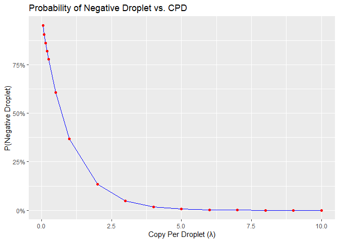
Probability of a Negative Droplet vs. CPD
We can also explore how the probability of a negative droplet (\(P(X = 0)\)) decreases as CPD (\(\lambda\)) increases:
cpd.list <- c(0.05, 0.1, 0.15, 0.2, 0.25,
              0.5, 1, 2, 3, 4, 5, 6, 7, 8, 9, 10)

prob <- round(exp(-cpd.list), 7)
df_prob <- data.frame(CPD = cpd.list,
                      P_negative = prob)

df_prob
## CPD P_negative
## 1 0.05 0.9512294
## 2 0.10 0.9048374
## 3 0.15 0.8607080
## 4 0.20 0.8187308
## 5 0.25 0.7788008
## 6 0.50 0.6065307
## 7 1.00 0.3678794
## 8 2.00 0.1353353
## 9 3.00 0.0497871
## 10 4.00 0.0183156
## 11 5.00 0.0067379
## 12 6.00 0.0024788
## 13 7.00 0.0009119
## 14 8.00 0.0003355
## 15 9.00 0.0001234
## 16 10.00 0.0000454Example values:
| CPD (λ) | P(Negative Droplet) |
|---|---|
| 0.05 | 0.9512294 |
| 0.25 | 0.7788008 |
| 1 | 0.3678794 |
| 3 | 0.0497871 |
| 5 | 0.0067379 |
| 10 | 0.0000454 |
Visualization
library(ggplot2)

ggplot(df_prob, aes(x = CPD, y = P_negative)) +
  geom_line(color = "blue") +
  geom_point(color = "red") +
  scale_y_continuous(labels = scales::percent) +
  labs(title = "Probability of Negative Droplet vs. CPD",
       x = "Copy Per Droplet (λ)",
       y = "P(Negative Droplet)")
Figure 3: Probability of negative droplet vs cpd
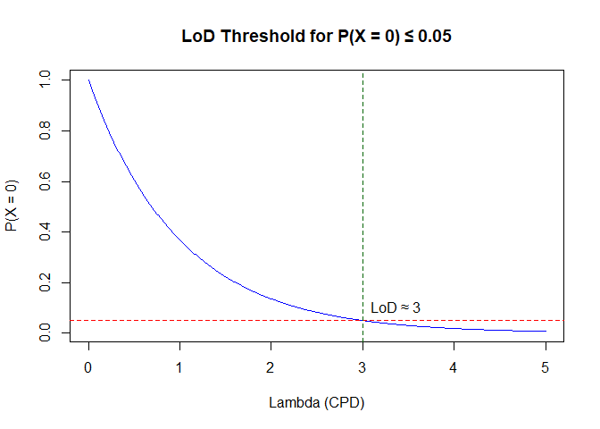
We also can define the Limit of Detection (LoD) as the lowest CPD (λ) where the probability of a negative droplet falls below a threshold (e.g., 5%).
alpha <- 0.05  # maximum acceptable false negative probability
lambda_seq <- seq(0, 5, by = 0.01)
p0 <- exp(-lambda_seq)
lod_lambda <- lambda_seq[which(p0 <= alpha)[1]]
lod_lambda
## [1] 3This means that at least 3 copies per droplet are needed to ensure that the probability of getting no signal at all is below 5%.
plot(lambda_seq, p0, type = "l", col = "blue",
     ylab = "P(X = 0)", xlab = "Lambda (CPD)",
     main = "LoD Threshold for P(X = 0) ≤ 0.05")
abline(h = alpha, col = "red", lty = 2)
abline(v = lod_lambda, col = "darkgreen", lty = 2)
text(lod_lambda, alpha + 0.05, paste0("LoD ≈ ", lod_lambda), pos = 4)
Figure 4: lod threshold
Interpretation
- When \(\lambda\) is small (e.g., 0.05), almost all droplets are negative.
- As \(\lambda\) increases, the probability of a droplet containing at least one copy increases rapidly.
- At \(\lambda = 3\), only ~5% of droplets are negative.
This relationship is critical when defining detection thresholds.
Application to ddPCR LoD
One way to define Limit of Detection (LoD) is to set a minimum \(\lambda\) such that:
\[ P(\text{No Detection}) = P(X=0) ≤ \alpha \] For example:
If we define \(\alpha = 0.05\), then LoD occurs around \(\lambda = 3\).
Summary
The Poisson model connects CPD with the likelihood of detecting target molecules.
This is essential for designing sensitive assays, particularly when working with low-abundance targets.
Next, we will explore how to calculate confidence intervals for \(\lambda\) and the resulting copy number.