Chapter 2: Binomial Distribution
A binomial distribution describes the number of successes in a fixed number of independent Bernoulli trials, each with the same probability of success \(p\).
We write: \[ X \sim B(n, p) \]
where:
\(n\) is the number of trials (e.g., number of droplets in ddPCR),
\(p\) is the probability of success in each trial,
\(X\) is the number of successful trials (positive droplets).
Example
Let’s consider a simple example using dice. Suppose we roll a die 3 times and count how many times we get a multiple of 3 (i.e., 3 or 6).
This is a Bernoulli trial repeated 3 times, with:
\[ p = \frac{2}{6} = \frac{1}{3}, \quad n = 3 \]
We are interested in the distribution of \(X\) = number of successes (i.e., times we get a 3 or 6).
The binomial probability mass function is:
\[ P(X = x) = \binom{n}{x} p^x (1 - p)^{n - x} \]
R Example: Computing Probabilities
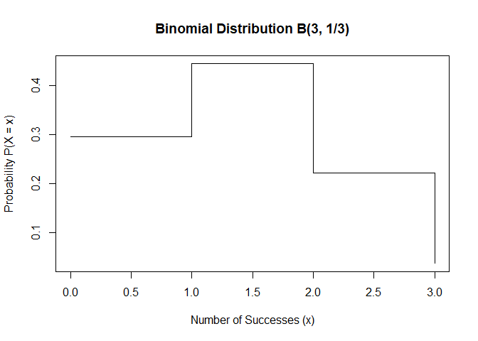
## [1] 0.29629630 0.44444444 0.22222222 0.03703704These correspond to:
\(P(X = 0)\) = 0.296 (no successes)
\(P(X = 1)\) = 0.444 (one success)
\(P(X = 2)\) = 0.222 (two successes)
\(P(X = 3)\) = 0.037 (all three are successes)
Visualizing the Binomial Distribution

Figure 1.1: binominal distribution
Interpretation in ddPCR
In ddPCR, each droplet is a Bernoulli trial: either positive or negative for the target DNA. When considering multiple droplets, the total number of positive droplets follows a binomial distribution. This distribution becomes particularly useful when modeling the number of positive droplets across many replicates, before transitioning to Poisson-based modeling for rare events.