Chapter 3: Analytical Similarity for Potency Assay Using TOST
Limitation of TOSTER package in R
While the TOSTER package offers a convenient and user-friendly way to conduct equivalence testing, it assumes equal variances by default and does not support flexible adjustments for unequal sample sizes or variance heterogeneity.
In real-world applications—particularly in biosimilar or analytical similarity studies—test and reference groups often differ in both size and variability. For example, the reference product may have a large, established data set with minimal variability, while the test product might be limited in size and exhibit different dispersion characteristics.
To account for these practical challenges, we implemented a custom function tost_auto_var_equal(), which:
Automatically checks variance equality using Levene’s test
Applies pooled or Welch-adjusted degrees of freedom as needed
Allows asymmetric sample sizes and includes RLD-based adjustments
Computes one-sided t-tests and confidence intervals consistent with the TOST framework
For this custom implementation, the following equations are used internally to compute the standard error, degrees of freedom, and confidence intervals, depending on the sample size and variance assumptions:
Equal sample size and variance
\[ SE_{\text{equal}} = \sqrt{ \frac{ \sigma_1^2 + \sigma_2^2 }{n} } \]
\[ df_{\text{equal}} = n_1 + n_2 - 2 \]
\[ CI = \delta \pm t_{1-\alpha, df_{\text{equal}}} \times SE_{\text{equal}} \]
Unequal sample size and equal variance
\[ s_p^2 = \frac{ (n_1 - 1)\sigma_1^2 + (n_2 - 1)\sigma_2^2 }{ n_1 + n_2 - 2 } \]
\[ SE_{\text{pooled}} = \sqrt{ s_p^2 \left( \frac{1}{n_1} + \frac{1}{n_2} \right) } \]
\[ df_{\text{pooled}} = n_1 + n_2 - 2 \]
\[ CI = \delta \pm t_{1-\alpha, df_{\text{pooled}}} \times SE_{\text{pooled}} \]
Unequal variance
\[ SE_{\text{Welch}} = \sqrt{ \frac{\sigma_1^2}{n_1} + \frac{\sigma_2^2}{n_2} } \]
\[ df_{\text{Welch}} = \frac{ \left( \frac{\sigma_1^2}{n_1} + \frac{\sigma_2^2}{n_2} \right)^2 } { \frac{ \sigma_1^4 }{ n_1^2 (n_1 - 1) } + \frac{ \sigma_2^4 }{ n_2^2 (n_2 - 1) } } \]
\[ CI = \delta \pm t_{1-\alpha, df_{\text{Welch}}} \times SE_{\text{Welch}} \]
| Symbol | Meaning |
|---|---|
| \(\delta\) | Mean difference: \(\bar{x}_1 - \bar{x}_2\) |
| \(\sigma_1^2, \sigma_2^2\) | Sample variances (groups 1 and 2) |
| \(n_1, n_2\) | Sample sizes for test and reference groups |
| \(df\) | Degrees of freedom |
| \(t_{1-\alpha, df}\) | Critical t value at 90% CI (one-sided α=0.05) |
TOST in Real World Application
To demonstrate how the custom tost_auto_var_equal() function works in practice, we simulate a simple example of potency testing where the test product has fewer available samples than the reference product since in potency testing for lot release or comparability studies, it is common that test samples are limited in number, while reference samples are more readily available.
Regulatory authorities, including the US FDA, permit the use of TOST to evaluate analytical similarity, even in the presence of sample size imbalance and variance heterogeneity, while allowing an excessively large RLD sample size can artificially narrow the confidence interval, leading to potentially biased conclusions regarding equivalence.
To mitigate this, regulatory guidance and internal validation practices often recommend limiting the effective sample size of the reference group. One commonly used rule is to cap the RLD sample size at 1.5 times that of the test group.
It is also common to use a margin of ±1.5 times the standard deviation of the reference group (SDref). This approach accounts for the biological variability of the assay and is widely accepted in practice (e.g., USP <1033>, bioassay validation guidelines), such as:
Therefore we can create simulation data set and set the equivalence margin such as:
set.seed(123)

# Reference: ample supply
group_ref <- rnorm(30, mean = 100, sd = 2)

# Test: limited availability
group_test <- rnorm(20, mean = 99, sd = 2)
and
# Reference mean and SD
ref_mean <- mean(group_ref)
ref_sd <- sd(group_ref)

# Raw to ratio scale
margin_raw <- 1.5*ref_sd
We then apply the custom function to assess equivalence:
tost_auto_var_equal <- function(g1, g2, margin_raw, alpha = 0.05, var.equal = NULL) {

  # Sample sizes
  n1 <- length(g1)  # Test (e.g., biosimilar or new lot)
  n2 <- length(g2)  # Reference (e.g., RLD or existing lot)

  # Variance assumption: automatic or user-specified
  if (is.null(var.equal)) {
    combined <- data.frame(
      value = c(g1, g2),
      group = factor(rep(c("g1", "g2"), times = c(n1, n2)))
    )
    # Levene’s test (robust to non-normality)
    p_var <- car::leveneTest(value ~ group, data = combined)[1, "Pr(>F)"]
    var_equal <- p_var > 0.05
  } else {
    var_equal <- var.equal
    p_var <- NA
  }

  # Group means, variances, and difference (delta)
  mean1 <- mean(g1)
  mean2 <- mean(g2)
  var1 <- var(g1)
  var2 <- var(g2)
  delta <- mean1 - mean2

   # Standard error (SE) and degrees of freedom (df)
  if (var_equal && n1 == n2) {
    se_diff <- sqrt((var1 + var2) / n1)
    df <- n1 + n2 - 2
    message("Equal variance & equal sample size")
  } else if (var_equal && n1 != n2) {
    n2 <- min(1.5 * n1, n2)  # RLD adjustment
    se_pooled <- ((n1 - 1) * var1 + (n2 - 1) * var2) / (n1 + n2 - 2)
    se_diff <- sqrt(se_pooled * (1 / n1 + 1 / n2))
    df <- n1 + n2 - 2
    message("Equal variance & unequal sample size (RLD adjusted)")
  } else {
    if (n1 != n2) {
      n2 <- min(1.5 * n1, n2)  # RLD adjustment
      message("Unequal variance & unequal sample size (RLD adjusted)")
    } else {
      message("Unequal variance & equal sample size")
    }
    se_diff <- sqrt(var1 / n1 + var2 / n2)
    df_num <- (var1 / n1 + var2 / n2)^2
    df_den <- (var1^2 / (n1^2 * (n1 - 1))) + (var2^2 / (n2^2 * (n2 - 1)))
    df <- df_num / df_den
  }


  # TOST one-sided t.tests
  t1 <- (delta + margin_raw) / se_diff
  t2 <- (delta - margin_raw) / se_diff
  p1 <- pt(t1, df, lower.tail = FALSE)
  p2 <- pt(t2, df, lower.tail = TRUE)

  # 90% Confidence Interval
  t_crit <- qt(1 - alpha, df)
  ci_lower <- delta - t_crit * se_diff
  ci_upper <- delta + t_crit * se_diff
  ci_raw_diff <- paste0(round(ci_lower, 3), " – ", round(ci_upper, 3))
  ci_within_margin <- (ci_lower >= -margin_raw) & (ci_upper <= margin_raw)

  # Result table
  tibble::tibble(
    delta = delta,
    t1 = t1, p1 = p1,
    t2 = t2, p2 = p2,
    CI_lower = ci_lower,
    CI_upper = ci_upper,
    margin_used = round(margin_raw, 4),
    df = round(df, 2),
    variance_equal = var_equal,
    variance_test_p = p_var,
    variance_assumption = if (var_equal) {
      "Equal variance assumed (Levene’s test p > 0.05)"
    } else {
      "Unequal variance assumed (Levene’s test p <= 0.05, Welch’s df applied)"
    },
    pass_equivalence = (p1 < alpha) & (p2 < alpha)
  )
}
The custom function above automatically determines whether to assume equal or unequal variances via Levene’s test, applies the correct degrees of freedom (pooled or Welch-adjusted), and limits the effective reference sample size to 1.5× that of the test group to avoid artificially narrow confidence intervals.
We can run the function and save the result as shown below:
## Equal variance & unequal sample size (RLD adjusted)We can summarize the results with the following helper function:
summarize_tost_result <- function(result_tost) {
  cat("=== TOST Summary ===\n")
  cat("Difference (delta):", round(result_tost$delta, 4), "\n")
  cat("90% CI: [", round(result_tost$CI_lower, 4), ",", round(result_tost$CI_upper, 4), "]\n")
  cat("Equivalence margin: ±", round(result_tost$margin_used, 4), "\n")
  cat("Degrees of freedom:", result_tost$df, "\n")
  cat("Variance assumption:", result_tost$variance_assumption, "\n")
  cat("TOST p-values: p1 =", round(result_tost$p1, 4), ", p2 =", round(result_tost$p2, 4), "\n")
  cat("=> Equivalence achieved? ", ifelse(result_tost$pass_equivalence, "YES", "NO"), "\n")
}## === TOST Summary ===
## Difference (delta): -0.5925
## 90% CI: [ -1.4929 , 0.308 ]
## Equivalence margin: ± 2.9431
## Degrees of freedom: 48
## Variance assumption: Equal variance assumed (Levene’s test p > 0.05)
## TOST p-values: p1 = 0 , p2 = 0
## => Equivalence achieved? YESAnd visualize the confidence interval compared to the equivalence margin:
library(ggplot2)

diff <- round(result_tost$delta, 4)
df_ci <- data.frame(lower = round(result_tost$CI_lower, 4),
                    upper = round(result_tost$CI_upper, 4),
                    mean_diff = diff,
                    e.margin = margin_raw)

ggplot(df_ci) +
  geom_errorbarh(aes(y = 1, xmin = lower, xmax = upper),
                 height = 0.1,   #
                 linewidth = 0.2) +
  geom_point(aes(y = 1, x = mean_diff), size = 3, color = "blue") +
  geom_vline(xintercept = c(-df_ci$e.margin, df_ci$e.margin), linetype = "dashed", color = "red", linewidth = 0.5) +
  xlim(-df_ci$e.margin-0.1, df_ci$e.margin+0.1) +
  ylim(0.5, 1.5) +
  labs(title = "Equivalence Testing: Confidence Interval vs Margin",
       x = "Difference in Means", y = "") +
  theme_minimal() +
  theme(axis.text.y = element_blank(),
        axis.ticks.y = element_blank())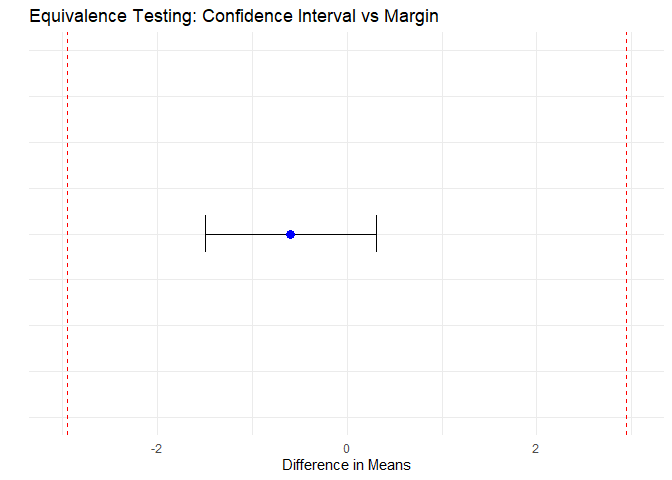
Figure 2: Equivalence Testing: Confidence Interval vs Margin
Conclusion
Based on the observed data:
The difference between test and reference is –0.5925, indicating the test product is slightly lower on average, but very close to the reference.
The 90% confidence interval of the difference is [–1.4929, 0.308].
The equivalence margin was calculated from the ±1.5 SD criterion as ±2.9431, and the observed CI is fully contained within this margin.
The degrees of freedom for the test were 48, reflecting adjustment for equal variances and unequal sample sizes, as determined by Levene’s test (p > 0.05).
TOST p-values were p1 = 0, p2 = 0, both well below α = 0.05.
Conclusion: The test product meets the equivalence criterion, demonstrating analytical similarity to the reference lot despite the sample size imbalance and variance difference.