Chapter 2: Application of TOST in R

In this chapter, we demonstrate how to apply the TOST procedure using R. We will use the TOSTER package, which provides user-friendly functions for equivalence testing.

Example Scenario

Suppose we are comparing the mean response of two treatment groups in a biosimilar study. We aim to determine whether the observed difference in means is small enough to be considered clinically negligible, i.e., within a pre-specified equivalence margin.

Let’s assume:

Group 1 (Test): Mean ≈ 100, SD ≈ 10
Group 2 (Reference): Mean ≈ 102, SD ≈ 10
Equivalence margin = ±5 units

Step 1: Simulated Data

set.seed(123)
group1 <- rnorm(30, mean = 100, sd = 10)
group2 <- rnorm(30, mean = 102, sd = 10)

summary(group1)

##    Min. 1st Qu.  Median    Mean 3rd Qu.    Max. 
##   80.33   93.29   99.26   99.53  104.89  117.87

summary(group2)

##    Min. 1st Qu.  Median    Mean 3rd Qu.    Max. 
##   86.51   98.97  102.48  103.78  109.57  123.69

Step 2: Traditional t-test (for comparison)

t.test(group1, group2)

## 
##  Welch Two Sample t-test
## 
## data:  group1 and group2
## t = -1.8087, df = 56.559, p-value = 0.07581
## alternative hypothesis: true difference in means is not equal to 0
## 95 percent confidence interval:
##  -8.9654261  0.4565843
## sample estimates:
## mean of x mean of y 
##  99.52896 103.78338

The p-value > 0.05 does not confirm equivalence, only that no significant difference was found.

Step 3: TOST Analysis with TOSTER

We now perform TOST with equivalence bounds of -5 and +5 units.

library(TOSTER)

TOST_result <- TOSTtwo.raw(m1 = mean(group1),
                           m2 = mean(group2),
                           sd1 = sd(group1),
                           sd2 = sd(group2),
                           n1 = length(group1),
                           n2 = length(group2),
                           low_eqbound = -5,
                           high_eqbound = 5,
                           alpha = 0.05)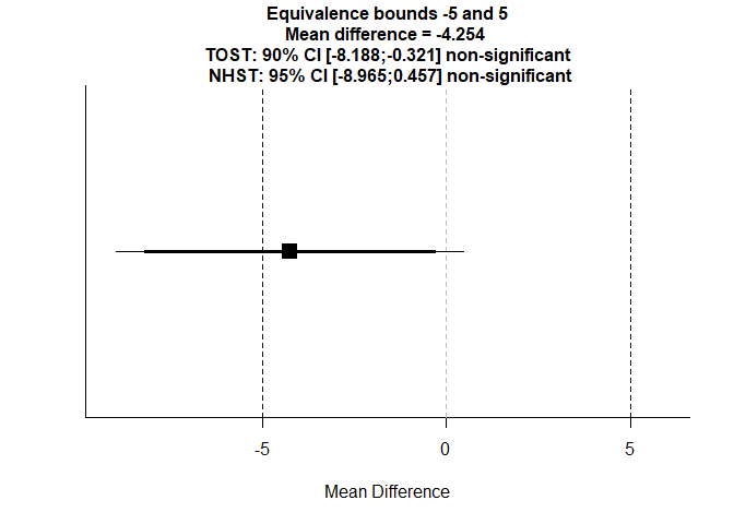

## TOST results:
## t-value lower bound: 0.317   p-value lower bound: 0.376
## t-value upper bound: -3.93   p-value upper bound: 0.0001
## degrees of freedom : 56.56
## 
## Equivalence bounds (raw scores):
## low eqbound: -5 
## high eqbound: 5
## 
## TOST confidence interval:
## lower bound 90% CI: -8.188
## upper bound 90% CI:  -0.321
## 
## NHST confidence interval:
## lower bound 95% CI: -8.965
## upper bound 95% CI:  0.457
## 
## Equivalence Test Result:
## The equivalence test was non-significant, t(56.56) = 0.317, p = 0.376, given equivalence bounds of -5.000 and 5.000 (on a raw scale) and an alpha of 0.05.

##

## 
## Null Hypothesis Test Result:
## The null hypothesis test was non-significant, t(56.56) = -1.809, p = 0.0758, given an alpha of 0.05.

##

## NHST: don't reject null significance hypothesis that the effect is equal to 0 
## TOST: don't reject null equivalence hypothesis

print(TOST_result)

## $diff
## [1] -4.254421
## 
## $TOST_t1
## [1] 0.3169703
## 
## $TOST_p1
## [1] 0.3762166
## 
## $TOST_t2
## [1] -3.934361
## 
## $TOST_p2
## [1] 0.0001152633
## 
## $TOST_df
## [1] 56.55858
## 
## $alpha
## [1] 0.05
## 
## $low_eqbound
## [1] -5
## 
## $high_eqbound
## [1] 5
## 
## $LL_CI_TOST
## [1] -8.187882
## 
## $UL_CI_TOST
## [1] -0.3209598
## 
## $LL_CI_TTEST
## [1] -8.965426
## 
## $UL_CI_TTEST
## [1] 0.4565843
## 
## $NHST_t
## [1] -1.808695
## 
## $NHST_p
## [1] 0.075815

Interpretation

If both one-sided p-values < 0.05, equivalence is concluded.
Check whether the 90% confidence interval lies entirely within [-5, +5]

Step 4: Visualizing Equivalence

library(ggplot2)

diff <- mean(group1) - mean(group2)
se <- sqrt(sd(group1)^2/length(group1) + sd(group2)^2/length(group2))
ci <- c(diff - qt(0.95, df=length(group1)+length(group2)-2)*se,
        diff + qt(0.95, df=length(group1)+length(group2)-2)*se)

df_ci <- data.frame(lower = ci[1], upper = ci[2], mean_diff = diff)

ggplot(df_ci) +
  geom_errorbarh(aes(y = 1, xmin = lower, xmax = upper), 
                 height = 0.1,   # 
                 linewidth = 0.2) +
  geom_point(aes(y = 1, x = mean_diff), size = 3, color = "blue") +
  geom_vline(xintercept = c(-5, 5), linetype = "dashed", color = "red", linewidth = 0.5) +
  xlim(-10, 10) +
  ylim(0.5, 1.5) +  
  labs(title = "Equivalence Testing: Confidence Interval vs Margin",
       x = "Difference in Means", y = "") +
  theme_minimal() +
  theme(axis.text.y = element_blank(),
        axis.ticks.y = element_blank())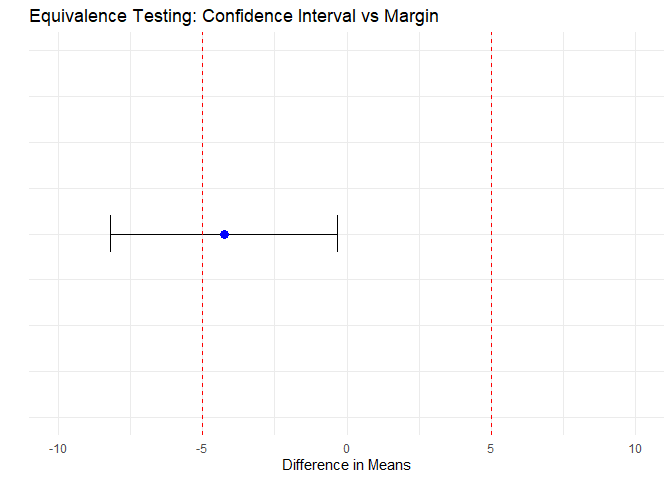

Figure 1: Equivalence Testing: Confidence Interval vs Margin

The confidence interval does not lie within the red dashed lines (equivalence margin) and therefore equivalence is not supported.

Manual TOST in R

For education purpose, we replicate the TOST calculation manually, using the same data.

Step 1: Mean difference and standard error

mean_diff <- mean(group1) - mean(group2)  
sd1 <- sd(group1)
sd2 <- sd(group2)
n1 <- length(group1)
n2 <- length(group2)
se_diff <- sqrt(sd1^2/n1 + sd2^2/n2)

Step 2: Degrees of freedom and critical t-value

# Welch-Satterthwaite approximation
df <- (sd1^2/n1 + sd2^2/n2)^2 / 
      ((sd1^4)/((n1-1)*n1^2) + (sd2^4)/((n2-1)*n2^2))

t_crit <- qt(0.95, df)  # For 90% CI

Step 3: Confidence interval of the difference

lci <- mean_diff - t_crit * se_diff
uci <- mean_diff + t_crit * se_diff

cat("90% CI: [", round(lci, 2), ",", round(uci, 2), "]\n")

## 90% CI: [ -8.19 , -0.32 ]

Step 4: Compare CI to Equivalence Margins

margin <- 5
if (lci > -margin & uci < margin) {
  cat("Conclusion: Equivalence supported.\n")
} else {
  cat("Conclusion: Equivalence NOT supported.\n")
}

## Conclusion: Equivalence NOT supported.

This manual approach yields the same conclusion as the TOSTER package.

Summary Table

Metric	Value
Mean difference	-4.25
90% Confidence Interval	[-8.19 ; -0.32]
Equivalence Margin	±5
Equivalence Conclusion	Not equivalent based on CI