Chapter 3: Impact of Ignoring LPC Variance on the True Failure Rate
Even though the FDA’s 1% rule defines a clear statistical target, the practical failure probability depends critically on how we treat the LPC variance (σ²_LPC).
If we assume that only the SCP variance matters (i.e., treat CP as fixed), we effectively underestimate total uncertainty — which can lead to fluctuating failure rates from run to run.
The following illustration demonstrates this effect using simulated normal distributions for SCP and LPC under different variance assumptions.
1. Concept and Setup
Let
\[
CP = \mu_{SCP} + z_{0.99}\sigma_{SCP}
\]
be the 99th percentile of the SCP distribution — the shared decision boundary.
For LPC, three scenarios are considered:
| Case | σLPC | Description |
|---|---|---|
| Equal variance | σLPC = σSCP | Typical baseline |
| Smaller variance | σLPC < σSCP | Very precise LPC |
| Larger variance | σLPC > σSCP | High variability LPC |
Two LPC mean-setting rules are compared:
Combined variance design (recommended):
\[ \mu_{LPC} = CP + z_{0.99}\sqrt{\sigma_{SCP}^2+\sigma_{LPC}^2} \]Naïve design (incorrect):
\[ \mu_{LPC} = CP + z_{0.99}\sigma_{LPC} \] which ignores the variability of CP itself.
If σLPC differs from σSCP, the naïve approach no longer guarantees the intended 1% failure rate.
2. Interpretation
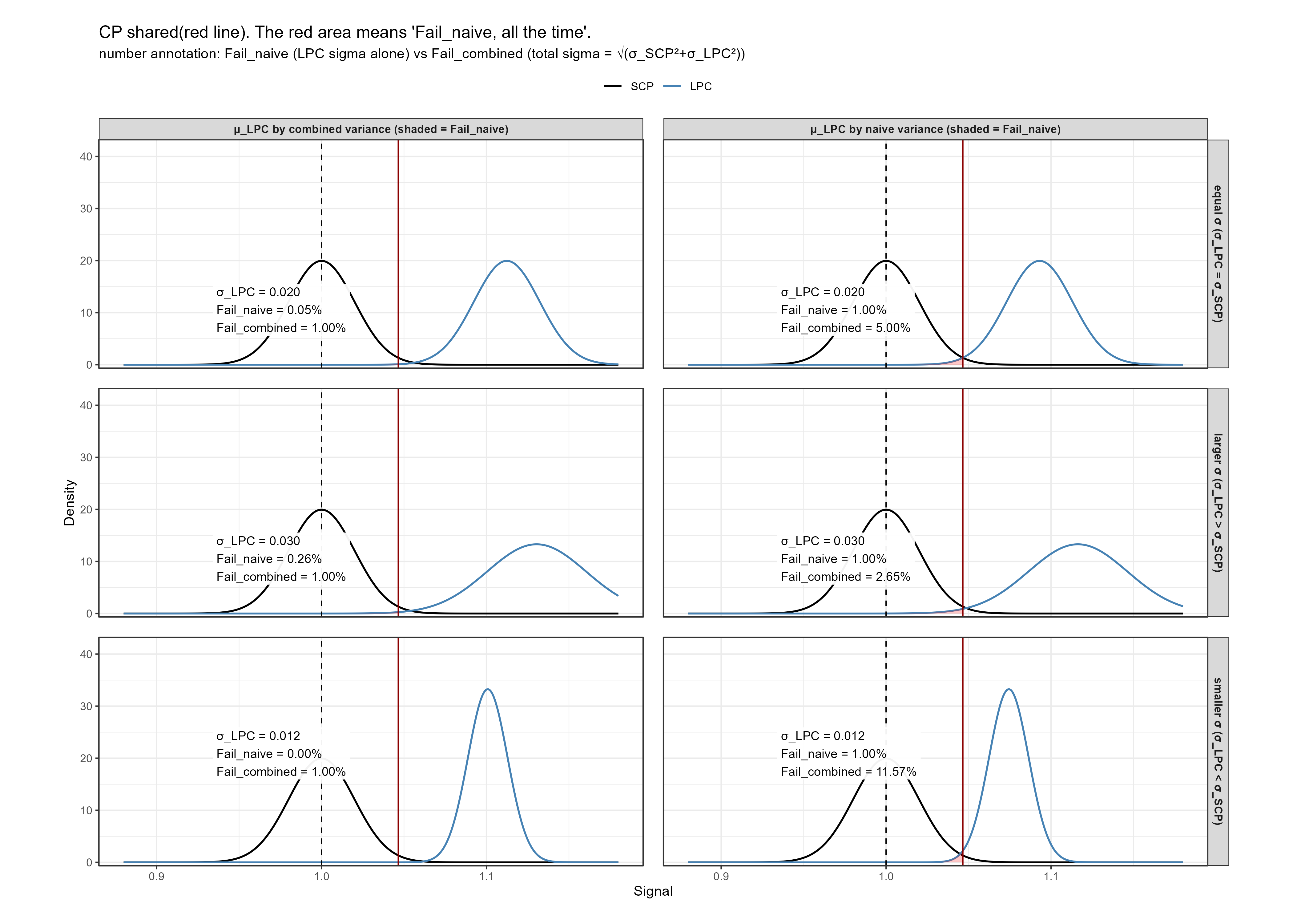
The panels show how the failure rate behaves under different assumptions:
Equal σ: Both approaches perform similarly, because total variance ≈ 2σ².
Smaller σLPC: The naïve method overestimates precision, setting μLPC too close to CP —the actual fail rate rises to >1%.
Larger σLPC: The naïve method overcompensates, placing μLPC too far right — resulting in fail rates well below 1%, making the assay unnecessarily insensitive.
This proves mathematically that the 1% rule is only stable when both variances are accounted for. Ignoring either σSCP or σLPC introduces run-to-run variability in the observed failure rate.
3. Theoretical Proof
Let
\[ CP \ = \ \mu_{SCP} \ + \ z_{0.99}\sigma_{SCP}, \quad \mu_{LPC} \ = \ CP \ + \ z_{0.99}\sigma_{LPC} \]
Then the true probability of LPC \(\le\) CP is:
\[ P(LPC \le CP) \ = \ \Phi(\frac{CP - \mu_{LPC}}{\sqrt{\sigma^2_{SCP} + \sigma^2_{LPC}}}) \ = \Phi(\frac{ -z_{0.99} \mu_{LPC}}{\sqrt{\sigma^2_{SCP} + \sigma^2_{LPC}}}) \]
Therefore, the combined-variance formula
\[ \mu_{LPC} \ = \ CP + z_{0.99}\sqrt{\sigma^2_{SCP} + \sigma^2_{LPC}} \]
is the only form that guarantees a stable 1% theoretical failure rate under independence.
4. Practical Implication
- Real assay systems always have nonzero σSCP and σLPC.
- If either component is ignored, the designed LPC may fail more (or less) often than intended.
- Observed variability in LPC pass/fail outcomes across validation runs is therefore a diagnostic indicator of whether the combined-variance principle was properly implemented.
In summary, the “1% fail” condition is not a property of the LPC itself, but of the joint SCP–LPC system.
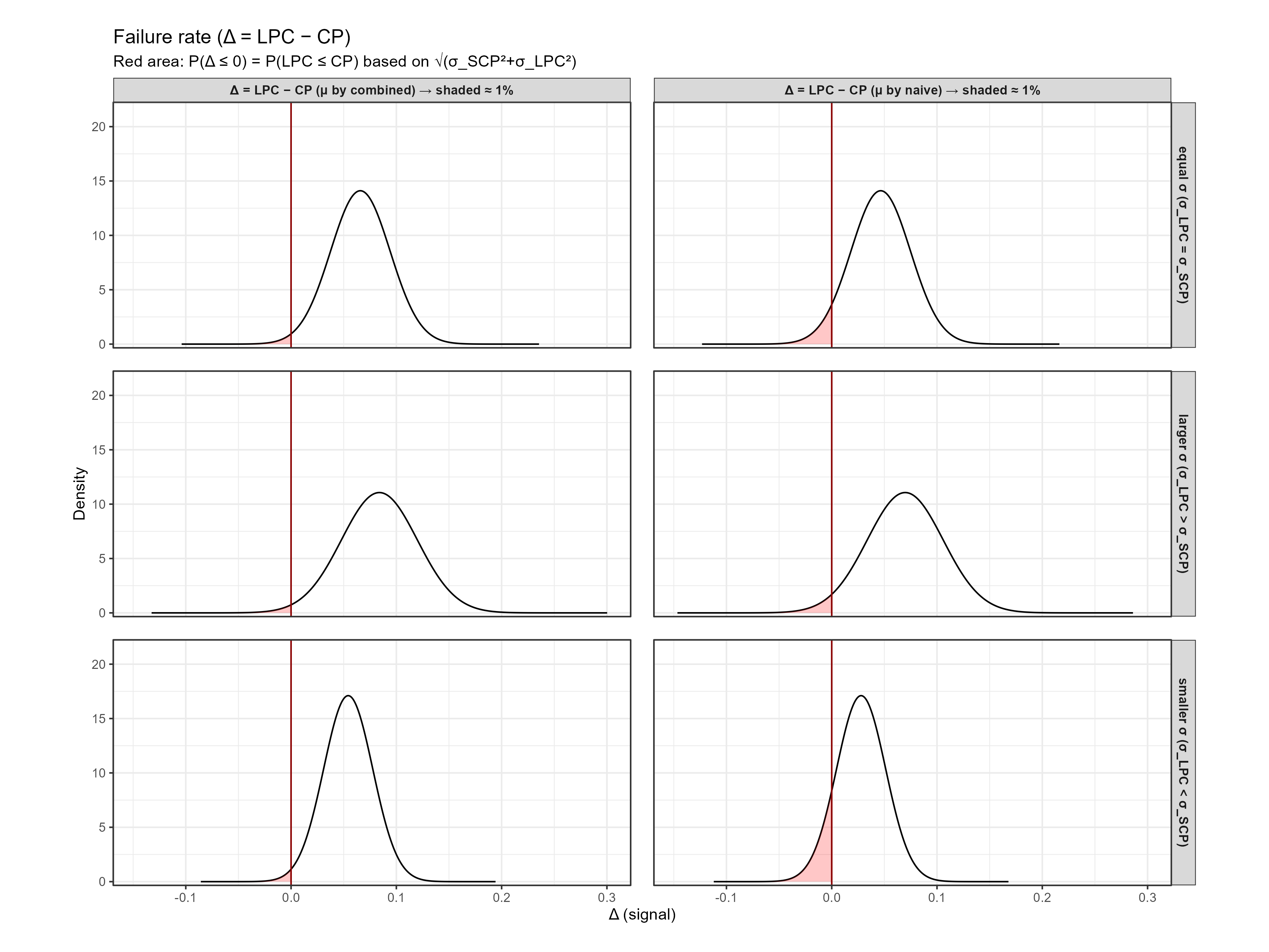
5. Optional Visualization of \(\triangle\) = LPC- CP Distribution
The difference variable
\[ \triangle \ = \ Y_{LPC} - CP \]
follows
\[ \triangle \sim N(\mu_{LPC} \ - \ CP, \ \sqrt{\sigma^2_{LPC}\ + \ \sigma^2_{SCP}}) \]
and failure corresponds to \(\triangle \le\) 0.
The following figure shows that when μLPC is set using the combined-variance approach, the shaded tail remains consistently \(\approx\) 1% regardless of σLPC.
Summary Points
- Treating CP as a fixed constant (ignoring σSCP) violates the definition of the 1% failure condition.
- The naïve formulas’ apparent simplicity hides a systematic bias that grows with σLPC.
- The combined-variance approach ensures theoretical consistency and empirical stability
- This distinction explains why observed LPC failure rates “Wander” even under well-controlled conditions — it is a mathematical inevitability when σ terms are mismatched.